

[ ]:
import pygeostat as gs
import numpy as np
import os
from matplotlib import pyplot as plt
Settings#
[ ]:
outdir = 'Output'
gs.mkdir(outdir)
#path to GSLIB executables
exe_dir="../pygeostat/executable/"

gs.PlotStyle['font.size'] = 12
gs.Parameters['data.tmin'] = -998
Loading data#
[ ]:
dfl = gs.ExampleData('point2d_surf')
dfl.head()
| HoleID | X | Y | Top Elevation | Thickness | Base Elevation | |
|---|---|---|---|---|---|---|
| 0 | 3.0 | 405.63 | 2135.75 | 376.69 | 47.98 | 328.71 |
| 1 | 5.0 | 235.89 | 1865.70 | 379.69 | 51.00 | 328.69 |
| 2 | 6.0 | 325.03 | 2055.81 | 376.86 | 49.34 | 327.52 |
| 3 | 7.0 | 675.54 | 2195.25 | 381.49 | 48.75 | 332.74 |
| 4 | 8.0 | 355.73 | 1995.74 | 376.97 | 48.94 | 328.03 |
[ ]:
dfl.info
DataFile: C:\Users\yimin\Anaconda3\envs\pygeostat\lib\site-packages\pygeostat\data\example_data\point2d_surf.dat
Attributes:
dh: 'HoleID',  x: 'X',  y: 'Y',
Variables:
'Top Elevation', 'Thickness', 'Base Elevation'
[ ]:
dfl.describe()
| Top Elevation | Thickness | Base Elevation | |
|---|---|---|---|
| count | 230.000000 | 230.000000 | 230.000000 |
| mean | 379.173739 | 50.096391 | 329.077348 |
| std | 2.607090 | 4.376842 | 4.571519 |
| min | 372.070000 | 37.730000 | 315.850000 |
| 25% | 377.222500 | 47.502500 | 327.137500 |
| 50% | 378.950000 | 49.390000 | 329.140000 |
| 75% | 380.782500 | 51.900000 | 332.225000 |
| max | 386.330000 | 62.870000 | 340.870000 |
Data Visualizations#
Distibution#
[ ]:
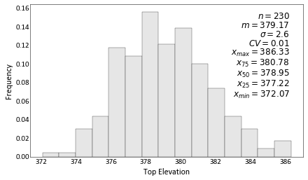
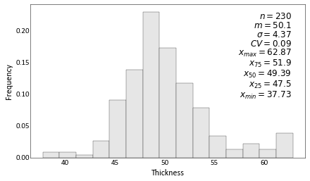
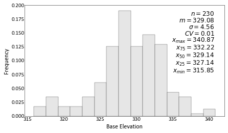
for var in dfl.variables:
    gs.histogram_plot(dfl, var=var, figsize = (7,4))
[ ]:
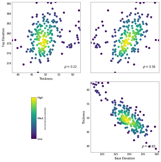
_ = gs.scatter_plots(dfl)
Location map#
[ ]:
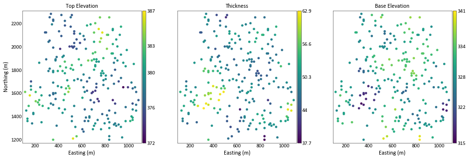
fig, axes = gs.subplots(1, len(dfl.variables), axes_pad=(0.9, 0.4), figsize= (25,5), cbar_mode='each', label_mode='L')
for i, var in enumerate(dfl.variables):
    gs.location_plot(dfl, var = var, ax = axes[i])
Normal Score Transformation#
[ ]:
nscore_p = gs.Program(program = exe_dir+'nscore', getpar=True)
C:\Users\yimin\Desktop\temp\pygeostat\pygeostat_public\examples\tmprdbr5twm\nscore.par has been copied to the clipboard
[ ]:
parstr = """      Parameters for NSCORE
                  *********************

START OF PARAMETERS:
{datafile}                -file with data
{n_var}  4 5 6           -  number of variables and columns
0                         -  column for weight, 0 if none
0                         -  column for category, 0 if none
0                         -  number of records if known, 0 if unknown
{tmin}   1.0e21          -  trimming limits
0                         -transform using a reference distribution, 1=yes
nofile.out                -file with reference distribution.
1   2   0                 -  columns for variable, weight, and category
201                       -maximum number of quantiles, 0 for all
{outfl}                -file for output
{trnfl}                -file for output transformation table
"""

nscore_outfl = os.path.join(outdir, 'nscore.out')

pars = dict(datafile=dfl.flname,
            tmin=gs.Parameters['data.tmin'],
            n_var = len(dfl.variables),
            outfl = nscore_outfl,
            trnfl = os.path.join(outdir, 'nscore.trn'))
nscore_p.run(parstr=parstr.format(**pars),quiet=True, liveoutput=True)
 NSCORE Version: 3.100

 data file = C:\Users\yimin\Anaconda3\envs\pygeostat\lib\site-packages\pygeostat\data\example_data\point2d_surf.dat
  columns =            4           5           6           0           0
  number of records =            0
  trimming limits =   -998.000000000000       1.000000000000000E+021
  consider a different reference dist =            0
  file with reference distribution = nofile.out
  columns =            1           2           0
  maximum number of quantiles =          201
  file for output = Output\nscore.out
  file for transformation table = Output\nscore.trn
 Determining size of C:\Users\yimin\Anaconda3\envs\pygeostat\lib\site-packages\pygeostat\data\example_data\point2d_surf.dat
 Reading C:\Users\yimin\Anaconda3\envs\pygeostat\lib\site-packages\pygeostat\data\example_data\point2d_surf.dat
 Building transform table   1 category   1
 Building transform table   2 category   1
 Building transform table   3 category   1
 Computing normal scores    1 category   1
 Computing normal scores    2 category   1
 Computing normal scores    3 category   1
 Generating output file
 Total execution time 0.050 seconds.

 NSCORE Version: 3.100 Finished
[ ]:
dfl_ns = gs.DataFile(nscore_outfl)
dfl_ns.head()
| HoleID | X | Y | Top Elevation | Thickness | Base Elevation | NS_Top Elevation | NS_Thickness | NS_Base Elevation | |
|---|---|---|---|---|---|---|---|---|---|
| 0 | 3.0 | 405.63 | 2135.75 | 376.69 | 47.98 | 328.71 | -0.92010 | -0.51919 | -0.13343 |
| 1 | 5.0 | 235.89 | 1865.70 | 379.69 | 51.00 | 328.69 | 0.24196 | 0.42938 | -0.14538 |
| 2 | 6.0 | 325.03 | 2055.81 | 376.86 | 49.34 | 327.52 | -0.82151 | -0.02331 | -0.51062 |
| 3 | 7.0 | 675.54 | 2195.25 | 381.49 | 48.75 | 332.74 | 0.87650 | -0.27596 | 0.82440 |
| 4 | 8.0 | 355.73 | 1995.74 | 376.97 | 48.94 | 328.03 | -0.77206 | -0.21829 | -0.39751 |
[ ]:
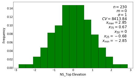
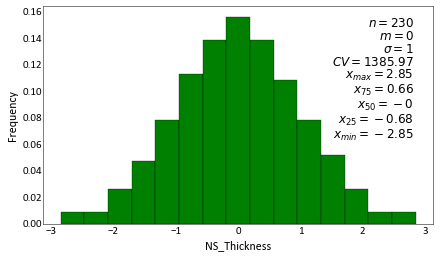
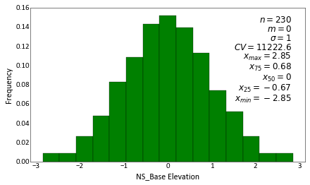
for var in dfl_ns.variables:
    if 'ns' in var.lower():
        gs.histogram_plot(dfl_ns, var=var, color='g', figsize = (7,4))
Variogram Calculation and Modeling#
[ ]:
dfl_ns.spacing(n_nearest=2)
dfl_ns.head()
| HoleID | X | Y | Top Elevation | Thickness | Base Elevation | NS_Top Elevation | NS_Thickness | NS_Base Elevation | Data Spacing (m) | |
|---|---|---|---|---|---|---|---|---|---|---|
| 0 | 3.0 | 405.63 | 2135.75 | 376.69 | 47.98 | 328.71 | -0.92010 | -0.51919 | -0.13343 | 57.952680 |
| 1 | 5.0 | 235.89 | 1865.70 | 379.69 | 51.00 | 328.69 | 0.24196 | 0.42938 | -0.14538 | 84.885990 |
| 2 | 6.0 | 325.03 | 2055.81 | 376.86 | 49.34 | 327.52 | -0.82151 | -0.02331 | -0.51062 | 40.660709 |
| 3 | 7.0 | 675.54 | 2195.25 | 381.49 | 48.75 | 332.74 | 0.87650 | -0.27596 | 0.82440 | 36.354945 |
| 4 | 8.0 | 355.73 | 1995.74 | 376.97 | 48.94 | 328.03 | -0.77206 | -0.21829 | -0.39751 | 62.080596 |
Horizonal variogram parameters#
[ ]:
lag_length_h = dfl_ns['Data Spacing (m)'].values.mean()
print('average data spacing in XY plane: {:.3f} {}'.format(lag_length_h,
                                                           gs.Parameters['plotting.unit']))
average data spacing in XY plane: 42.812 m
[ ]:
x_range = np.ptp(dfl[dfl.x].values)
y_range = np.ptp(dfl[dfl.y].values)
n_lag_x =  np.ceil((x_range * 0.5) /  lag_length_h)
n_lag_y =  np.ceil((y_range * 0.5) /  lag_length_h)
lag_tol_h = lag_length_h * 0.6
[ ]:
var_calc = gs.Program(program=exe_dir+'varcalc')
[ ]:
parstr = """      Parameters for VARCALC
                  **********************

START OF PARAMETERS:
{file}                             -file with data
2 3 0                              -   columns for X, Y, Z coordinates
1 7                                -   number of variables,column numbers (position used for tail,head variables below)
{t_min}    1.0e21                   -   trimming limits
{n_directions}                                  -number of directions
0.0 15 1000 0.0 22.5 1000 0.0   -Dir 01: azm,azmtol,bandhorz,dip,diptol,bandvert,tilt
 {n_lag_y}  {lag_length_h}  {lag_tol_h}            -        number of lags,lag distance,lag tolerance
90.0 15 1000 0.0 22.5 1000 0.0   -Dir 02: azm,azmtol,bandhorz,dip,diptol,bandvert,tilt
 {n_lag_x}  {lag_length_h}  {lag_tol_h}                 -        number of lags,lag distance,lag tolerance
{output}                          -file for experimental variogram points output.
0                                 -legacy output (0=no, 1=write out gamv2004 format)
1                                 -run checks for common errors
1                                 -standardize sills? (0=no, 1=yes)
1                                 -number of variogram types
1   1   1   1                     -tail variable, head variable, variogram type (and cutoff/category), sill
"""

n_directions = 2
varcalc_outfl = os.path.join(outdir, 'varcalc.out')

var_calc.run(parstr=parstr.format(file=dfl_ns.flname,
                                  n_directions = n_directions,
                                  t_min = gs.Parameters['data.tmin'],
                                  n_lag_x=n_lag_x,
                                  n_lag_y=n_lag_y,
                                  lag_length_h = lag_length_h,
                                  lag_tol_h = lag_tol_h,
                                  output=varcalc_outfl),
             liveoutput=True)
Calling:  ['../pygeostat/executable/varcalc', 'temp']

varcalc version:  1.400

  data file: Output\nscore.out
  x,y,z columns:            2           3           0
  number of variables:            1
  Variable columns:            7
  tmin,tmax:   -998.000000000000       1.000000000000000E+021
  number of directions:            2
  direction parameters:
 azm,azmtol,bandhorz  0.000000000000000E+000   15.0000000000000
   1000.00000000000
 dip,diptol,bandvert  0.000000000000000E+000   22.5000000000000
   1000.00000000000
 tilt  0.000000000000000E+000
 nlags,lagdist,lagtol          13   42.8115108947752
   25.6869065368651
 azm,azmtol,bandhorz   90.0000000000000        15.0000000000000
   1000.00000000000
 dip,diptol,bandvert  0.000000000000000E+000   22.5000000000000
   1000.00000000000
 tilt  0.000000000000000E+000
 nlags,lagdist,lagtol          12   42.8115108947752
   25.6869065368651
  output file: Output\varcalc.out
  legacy output?            0
  run checks?            1
  attempt to standardize sills?            1
  number of variogram types:            1
 Variogram tail,head,type           1           1           1
  standardizing with sill =   1.00000000000000
 Reading data file
 Setting up final parameters for variogram calculation
 Calculating variograms...
  working on direction            1
  working on direction            2
[ ]:
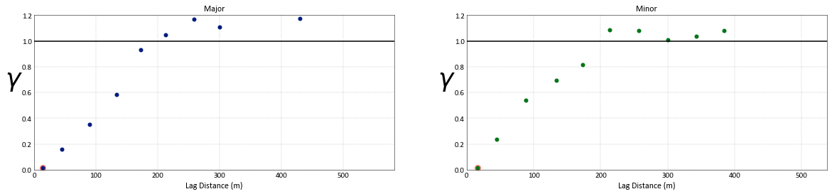
varfl = gs.DataFile(varcalc_outfl)
varfl.head()
| Variogram Index | Lag Distance | Number of Pairs | Variogram Value | Variogram Number | Calculation Azimuth | Calculation Dip | Variogram Type | Variogram Tail Index | Variogram Head Index | |
|---|---|---|---|---|---|---|---|---|---|---|
| 0 | 1.0 | 13.876815 | 13.0 | 0.012783 | 1.0 | 0.0 | 0.0 | 1.0 | 1.0 | 1.0 |
| 1 | 1.0 | 45.068702 | 54.0 | 0.160347 | 1.0 | 0.0 | 0.0 | 1.0 | 1.0 | 1.0 |
| 2 | 1.0 | 89.293385 | 135.0 | 0.349820 | 1.0 | 0.0 | 0.0 | 1.0 | 1.0 | 1.0 |
| 3 | 1.0 | 133.200325 | 160.0 | 0.582054 | 1.0 | 0.0 | 0.0 | 1.0 | 1.0 | 1.0 |
| 4 | 1.0 | 172.965087 | 220.0 | 0.929005 | 1.0 | 0.0 | 0.0 | 1.0 | 1.0 | 1.0 |
[ ]:
colors = gs.get_palette('cat_dark', n_directions, cmap=False)
titles = ['Major', 'Minor', 'Vertical']
fig, axes = plt.subplots(1, n_directions, figsize= (20,4))
for i in range(n_directions):
    gs.variogram_plot(varfl, index=i+1, ax = axes[i], color=colors[i], title = titles[i], grid=True)
[ ]:
var_model = gs.Program(program=exe_dir+'varmodel')
[ ]:
parstr = """      Parameters for VARMODEL
                  ***********************

START OF PARAMETERS:
{varmodel_outfl}             -file for modeled variogram points output
3                            -number of directions to model points along
0.0   0.0  100   25          -  azm, dip, npoints, point separation
90.0   0.0  100   15       -  azm, dip, npoints, point separation
0.0   90.0  100   0.2       -  azm, dip, npoints, point separation
2    0.05                   -nst, nugget effect
3    ?    0.0   0.0   0.0    -it,cc,azm,dip,tilt (ang1,ang2,ang3)
        ?     ?     ?    -a_hmax, a_hmin, a_vert (ranges)
3    ?    0.0   0.0   0.0    -it,cc,azm,dip,tilt (ang1,ang2,ang3)
        ?     ?     ?    -a_hmax, a_hmin, a_vert (ranges)
1   100000                   -fit model (0=no, 1=yes), maximum iterations
1.0                          -  variogram sill (can be fit, but not recommended in most cases)
1                            -  number of experimental files to use
{varcalc_outfl}              -    experimental output file 1
3 1 2 3                    -      # of variograms (<=0 for all), variogram #s
1   0   10                   -  # pairs weighting, inverse distance weighting, min pairs
0     10.0                   -  fix Hmax/Vert anis. (0=no, 1=yes)
0      1.0                   -  fix Hmin/Hmax anis. (0=no, 1=yes)
{varmodelfit_outfl}          -  file to save fit variogram model
"""

varmodel_outfl = os.path.join(outdir, 'varmodel.out')
varmodelfit_outfl = os.path.join(outdir, 'varmodelfit.out')

var_model.run(parstr=parstr.format(varmodel_outfl= varmodel_outfl,
                                   varmodelfit_outfl = varmodelfit_outfl,
                                   varcalc_outfl = varcalc_outfl), liveoutput=False, quiet=True)
[ ]:
varmdl = gs.DataFile(varmodel_outfl)
varmdl.head()
| Variogram Index | Lag Distance | Number of Pairs | Variogram Value | Variogram Number | Calculation Azimuth | Calculation Dip | |
|---|---|---|---|---|---|---|---|
| 0 | 1.0 | 25.0 | 1.0 | 0.088593 | 1.0 | 0.0 | 0.0 |
| 1 | 1.0 | 50.0 | 1.0 | 0.195217 | 1.0 | 0.0 | 0.0 |
| 2 | 1.0 | 75.0 | 1.0 | 0.345932 | 1.0 | 0.0 | 0.0 |
| 3 | 1.0 | 100.0 | 1.0 | 0.510735 | 1.0 | 0.0 | 0.0 |
| 4 | 1.0 | 125.0 | 1.0 | 0.663145 | 1.0 | 0.0 | 0.0 |
[ ]:
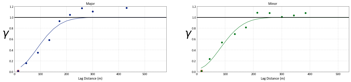
fig, axes = plt.subplots(1, n_directions, figsize= (20,4))
for i in range(n_directions):
    gs.variogram_plot(varfl, index=i+1, ax = axes[i], color=colors[i], title = titles[i], grid=True)
    gs.variogram_plot(varmdl, index=i+1, ax = axes[i], color=colors[i], experimental=False)
Kriging#
[ ]:
print(dfl_ns.infergriddef(nblk=[200,200,1]))
200 112.45 4.9
200 1202.725 5.45
1 0.5 1.0
[ ]:
kt3dn = gs.Program(exe_dir+'kt3dn', getpar=True)
C:\Users\yimin\Desktop\temp\pygeostat\pygeostat_public\examples\tmpb6q2f19a\kt3dn.par has been copied to the clipboard
[ ]:
parstr_ = """     Parameters for KT3DN
                 ********************
START OF PARAMETERS:
{file}                                -file with data
1  2 3 0 4 0                          -  columns for DH,X,Y,Z,var,sec var
{t_min}    1.0e21                     -  trimming limits
0                                     -option: 0=grid, 1=cross, 2=jackknife
nojack.out                           -file with jackknife data
0 0 0 0   0                          -   columns for X,Y,Z,vr and sec var
kt3dn_dataspacing.out                 -data spacing analysis output file (see note)
1    20.0                             -  number to search (0 for no dataspacing analysis, rec. 10 or 20) and composite length
0    100   0                          -debugging level: 0,3,5,10; max data for GSKV;output total weight of each data?(0=no,1=yes)
kt3dn.dbg-nkt3dn.sum                  -file for debugging output (see note)
{output}                              -file for kriged output (see GSB note)
{griddef}
1    1      1                         -x,y and z block discretization
20    80    12    1                    -min, max data for kriging,upper max for ASO,ASO incr
0      0                              -max per octant, max per drillhole (0-> not used)
500.0  500.0  150.0                   -maximum search radii
 0.0   0.0   0.0                      -angles for search ellipsoid
1                                     -0=SK,1=OK,2=LVM(resid),3=LVM((1-w)*m(u))),4=colo,5=exdrift,6=ICCK
0.0 0.6  0.8                          -  mean (if 0,4,5,6), corr. (if 4 or 6), var. reduction factor (if 4)
0 0 0 0 0 0 0 0 0                     -drift: x,y,z,xx,yy,zz,xy,xz,zy
0                                     -0, variable; 1, estimate trend
extdrift.out                          -gridded file with drift/mean
4                                     -  column number in gridded file
keyout.out                            -gridded file with keyout (see note)
0    1                                -  column (0 if no keyout) and value to keep
{varmodel}
"""


krig_output = os.path.join(outdir, 'KrigGrid.out')

with open(varmodelfit_outfl, 'r') as f:
    varmodel_ = f.readlines()
varmodel = ''''''
for line in varmodel_:
    varmodel += line


parstr=parstr_.format(file=dfl_ns.flname,
                     t_min = gs.Parameters['data.tmin'],
                      griddef = str(dfl_ns.griddef),
                     varmodel=varmodel,
                     output=krig_output)
kt3dn.run(parstr=parstr, liveoutput=True)
Calling:  ['../pygeostat/executable/kt3dn', 'temp']

 KT3DN Version: 7.4.1

  data file = Output\nscore.out
  columns =            1           2           3           0           4
           0
  trimming limits =   -998.000000000000       1.000000000000000E+021
  kriging option =            0
  jackknife data file = nojack.out
  columns =            0           0           0           0           0
  data spacing analysis output file = kt3dn_dataspacing.out
  debugging level =            0
  summary only file = kt3dn.sum
  debugging file = kt3dn.dbg
  GSLIB-style output file = Output\KrigGrid.out
  nx, xmn, xsiz =          200   112.450000000000        4.90000000000000
  ny, ymn, ysiz =          200   1202.72500000000        5.45000000000000
  nz, zmn, zsiz =            1  0.500000000000000        1.00000000000000
  block discretization:           1           1           1
  ndmin,ndmax =           20          80
  max per octant =            0
  max per drillhole =            0
  search radii =    500.000000000000        500.000000000000
   150.000000000000
  search anisotropy angles =   0.000000000000000E+000  0.000000000000000E+000
  0.000000000000000E+000
 Running data spacing analysis
 Number of search data and length of composites =           1
   20.0000000000000
  Building data spacing analysis table
  using ordinary kriging
  drift terms =            0           0           0           0           0
           0           0           0           0
  itrend =            0
  external drift file = extdrift.out
  GSLIB-style external grid file = extdrift.out
  column for external variable =            4
  keyout indicator file = keyout.out
  not applying keyout
  nst, c0 =            2  5.000000000000000E-002
  it,cc,ang[1,2,3];            3  0.940000000000000       0.000000000000000E+000
  0.000000000000000E+000  0.000000000000000E+000
  a1 a2 a3:    212.630000000000        200.410000000000
   278.150000000000
  it,cc,ang[1,2,3];            3  1.000000000000000E-002  0.000000000000000E+000
  0.000000000000000E+000  0.000000000000000E+000
  a1 a2 a3:    212.480000000000        197.450000000000
   556.300000000000
 Checking the data set for duplicates
  No duplicates found
 Data for KT3D: Variable number            4
   Number   =          230
   Average  =    379.173739130435
   Variance =    6.76736514930963
 Presorting the data along an arbitrary vector
 Data was presorted with angles:   12.5000000000000        12.5000000000000
   12.5000000000000
 Setting up rotation matrices for variogram and search
 Setting up super block search strategy

 Working on the kriging
   currently on estimate      4000
   currently on estimate      8000
   currently on estimate     12000
   currently on estimate     16000
   currently on estimate     20000
   currently on estimate     24000
   currently on estimate     28000
   currently on estimate     32000
   currently on estimate     36000
   currently on estimate     40000

 KT3DN Version:    7.4.1 Finished
[ ]:
krigfl = gs.DataFile(krig_output, griddef=dfl_ns.griddef)
krigfl.head()
| Estimate | EstimationVariance | |
|---|---|---|
| 0 | 380.15450 | 1.034023 |
| 1 | 379.85315 | 1.024630 |
| 2 | 379.77858 | 1.017963 |
| 3 | 379.73702 | 1.011976 |
| 4 | 379.61243 | 1.003637 |
[ ]:
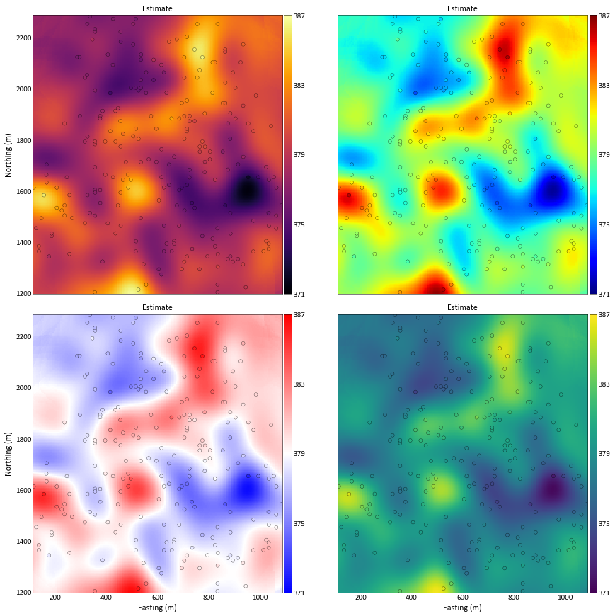
cmaps = ['inferno', 'jet', 'bwr', 'viridis']
fig, axes = gs.subplots(2, 2, axes_pad=(0.9, 0.4), figsize= (20,15), cbar_mode='each', label_mode='L')
for i, ax in enumerate(axes):
    gs.slice_plot(krigfl, var='Estimate', orient='xy', cmap=cmaps[i], ax=ax, pointdata=dfl_ns,
                  pointvar='Top Elevation', pointkws={'edgecolors':'k', 's':25})
[ ]:
# Clean up
try:
    gs.rmfile('kt3dn.sum')
    gs.rmfile('kt3dn.dbg')
    gs.rmfile('kt3dn_dataspacing.out')
    gs.rmfile('temp')
    gs.rmdir(outdir)
except:
    pass