

[ ]:
import pygeostat as gs
import numpy as np
import os
import pandas as pd
from matplotlib import pyplot as plt
Settings#
[ ]:
outdir = 'Output'
gs.mkdir(outdir)
#path to GSLIB executables
exe_dir="../pygeostat/executable/"

gs.PlotStyle['font.size'] = 12
gs.Parameters['data.tmin'] = -998
Loading data#
[ ]:
dfl = gs.ExampleData('point2d_mv')
dfl.head()
| X | Y | Var1 | Var2 | Var3 | |
|---|---|---|---|---|---|
| 0 | 28949.708226 | 96548.685172 | 0.78641 | 2.96716 | -1.47010 |
| 1 | 24610.158555 | 96251.877101 | 0.54300 | 2.13614 | 0.74573 |
| 2 | 27719.964681 | 90687.703337 | -0.39320 | 0.48682 | 0.23470 |
| 3 | 26910.320345 | 92501.863566 | 0.44938 | 1.27002 | -0.31840 |
| 4 | 21725.601294 | 92981.211253 | 1.38558 | 1.77734 | 2.40020 |
[ ]:
dfl.info
DataFile: C:\Users\yimin\Anaconda3\envs\pygeostat\lib\site-packages\pygeostat\data\example_data\point2d_mv.dat
Attributes:
x: 'X',  y: 'Y',
Variables:
'Var1', 'Var2', 'Var3'
Data Visualizations#
Distibution#
[ ]:
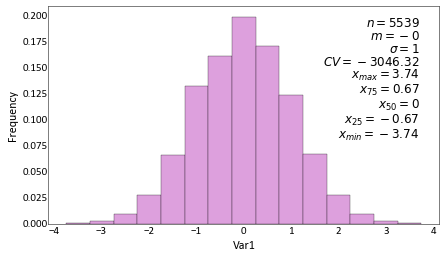
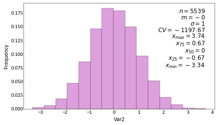
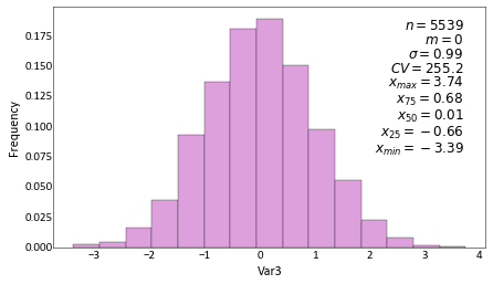
for var in dfl.variables:
    gs.histogram_plot(dfl, var=var, figsize = (7,4), color='plum')
[ ]:
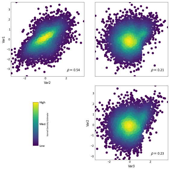
_ = gs.scatter_plots(dfl)
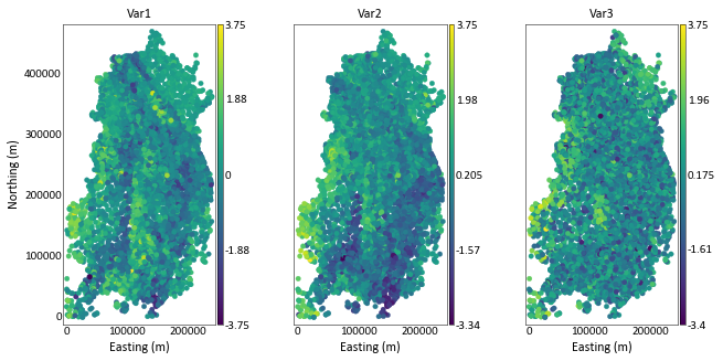
Location map#
[ ]:
fig, axes = gs.subplots(1, len(dfl.variables), axes_pad=(0.9, 0.4), figsize= (25,5), cbar_mode='each', label_mode='L')
for i, var in enumerate(dfl.variables):
    gs.location_plot(dfl, var = var, ax = axes[i])
Variogram Calculation and Modeling#
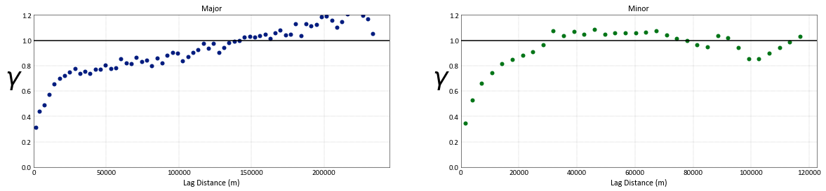
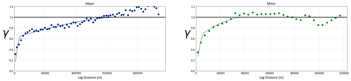
Experimental variogram is claulated and modeled for the first variable
[ ]:
dfl.spacing(n_nearest=5)
dfl.head()
WARNING: current implementation of function is likely too memory intensivefor greater than 5000 data
| X | Y | Var1 | Var2 | Var3 | Data Spacing (m) | |
|---|---|---|---|---|---|---|
| 0 | 28949.708226 | 96548.685172 | 0.78641 | 2.96716 | -1.47010 | 5313.903775 |
| 1 | 24610.158555 | 96251.877101 | 0.54300 | 2.13614 | 0.74573 | 3989.836067 |
| 2 | 27719.964681 | 90687.703337 | -0.39320 | 0.48682 | 0.23470 | 5051.373369 |
| 3 | 26910.320345 | 92501.863566 | 0.44938 | 1.27002 | -0.31840 | 3929.811601 |
| 4 | 21725.601294 | 92981.211253 | 1.38558 | 1.77734 | 2.40020 | 4054.581266 |
Horizonal variogram parameters#
[ ]:
lag_length_h = dfl['Data Spacing (m)'].values.mean()
print('average data spacing in XY plane: {:.3f} {}'.format(lag_length_h,
                                                           gs.Parameters['plotting.unit']))
average data spacing in XY plane: 3540.358 m
[ ]:
x_range = np.ptp(dfl[dfl.x].values)
y_range = np.ptp(dfl[dfl.y].values)
n_lag_x =  (x_range * 0.5) /  lag_length_h
n_lag_y =  (y_range * 0.5) /  lag_length_h
lag_tol_h = lag_length_h * 0.6
[ ]:
var_calc = gs.Program(program=exe_dir+'varcalc')
[ ]:
parstr = """      Parameters for VARCALC
                  **********************

START OF PARAMETERS:
{file}                             -file with data
1 2 0                              -   columns for X, Y, Z coordinates
1 3                                -   number of variables,column numbers (position used for tail,head variables below)
{t_min}    1.0e21                   -   trimming limits
{n_directions}                                  -number of directions
0.0 15 1000 0.0 22.5 1000 0.0   -Dir 01: azm,azmtol,bandhorz,dip,diptol,bandvert,tilt
 {n_lag_y}  {lag_length_h}  {lag_tol_h}            -        number of lags,lag distance,lag tolerance
90.0 15 1000 0.0 22.5 1000 0.0   -Dir 02: azm,azmtol,bandhorz,dip,diptol,bandvert,tilt
 {n_lag_x}  {lag_length_h}  {lag_tol_h}                 -        number of lags,lag distance,lag tolerance
{output}                          -file for experimental variogram points output.
0                                 -legacy output (0=no, 1=write out gamv2004 format)
1                                 -run checks for common errors
1                                 -standardize sills? (0=no, 1=yes)
1                                 -number of variogram types
1   1   1   1                     -tail variable, head variable, variogram type (and cutoff/category), sill
"""

n_directions = 2
varcalc_outfl = os.path.join(outdir, 'varcalc.out')

var_calc.run(parstr=parstr.format(file=dfl.flname,
                                  n_directions = n_directions,
                                  t_min = gs.Parameters['data.tmin'],
                                  n_lag_x=n_lag_x,
                                  n_lag_y=n_lag_y,
                                  lag_length_h = lag_length_h,
                                  lag_tol_h = lag_tol_h,
                                  output=varcalc_outfl),
             liveoutput=True)
Calling:  ['../pygeostat/executable/varcalc', 'temp']

varcalc version:  1.400

  data file:
 C:\Users\yimin\Anaconda3\envs\pygeostat\lib\site-packages\pygeostat\data\exampl
 e_data\point2d_mv.dat
  x,y,z columns:            1           2           0
  number of variables:            1
  Variable columns:            3
  tmin,tmax:   -998.000000000000       1.000000000000000E+021
  number of directions:            2
  direction parameters:
 azm,azmtol,bandhorz  0.000000000000000E+000   15.0000000000000
   1000.00000000000
 dip,diptol,bandvert  0.000000000000000E+000   22.5000000000000
   1000.00000000000
 tilt  0.000000000000000E+000
 nlags,lagdist,lagtol          66   3540.35845705671
   2124.21507423402
 azm,azmtol,bandhorz   90.0000000000000        15.0000000000000
   1000.00000000000
 dip,diptol,bandvert  0.000000000000000E+000   22.5000000000000
   1000.00000000000
 tilt  0.000000000000000E+000
 nlags,lagdist,lagtol          33   3540.35845705671
   2124.21507423402
  output file: Output\varcalc.out
  legacy output?            0
  run checks?            1
  attempt to standardize sills?            1
  number of variogram types:            1
 Variogram tail,head,type           1           1           1
  standardizing with sill =   1.00000000000000
 Reading data file
 Setting up final parameters for variogram calculation
 Calculating variograms...
  working on direction            1
  working on direction            2
[ ]:
varfl = gs.DataFile(varcalc_outfl)
varfl.head()
| Variogram Index | Lag Distance | Number of Pairs | Variogram Value | Variogram Number | Calculation Azimuth | Calculation Dip | Variogram Type | Variogram Tail Index | Variogram Head Index | |
|---|---|---|---|---|---|---|---|---|---|---|
| 0 | 1.0 | 1356.675118 | 468.0 | 0.310738 | 1.0 | 0.0 | 0.0 | 1.0 | 1.0 | 1.0 |
| 1 | 1.0 | 3873.560972 | 3070.0 | 0.438385 | 1.0 | 0.0 | 0.0 | 1.0 | 1.0 | 1.0 |
| 2 | 1.0 | 7071.060717 | 3893.0 | 0.490704 | 1.0 | 0.0 | 0.0 | 1.0 | 1.0 | 1.0 |
| 3 | 1.0 | 10611.610525 | 3662.0 | 0.574807 | 1.0 | 0.0 | 0.0 | 1.0 | 1.0 | 1.0 |
| 4 | 1.0 | 14141.319963 | 3558.0 | 0.656667 | 1.0 | 0.0 | 0.0 | 1.0 | 1.0 | 1.0 |
[ ]:
colors = gs.get_palette('cat_dark', n_directions, cmap=False)
titles = ['Major', 'Minor']
fig, axes = plt.subplots(1, n_directions, figsize= (20,4))
for i in range(n_directions):
    gs.variogram_plot(varfl, index=i+1, ax = axes[i], color=colors[i], title = titles[i], grid=True)
[ ]:
var_model = gs.Program(program=exe_dir+'varmodel')
[ ]:
parstr = """      Parameters for VARMODEL
                  ***********************

START OF PARAMETERS:
{varmodel_outfl}             -file for modeled variogram points output
{n_directions}                             -number of directions to model points along
0.0   0.0  {n_lag_y}  {lag_length_h}         -  azm, dip, npoints, point separation
90.0   0.0  {n_lag_x}  {lag_length_h}      -  azm, dip, npoints, point separation
2    0.0                   -nst, nugget effect
1    ?    0.0   0.0   0.0    -it,cc,azm,dip,tilt (ang1,ang2,ang3)
        ?     ?     ?    -a_hmax, a_hmin, a_vert (ranges)
1    ?    0.0   0.0   0.0    -it,cc,azm,dip,tilt (ang1,ang2,ang3)
        ?     ?     ?    -a_hmax, a_hmin, a_vert (ranges)
1   100000                   -fit model (0=no, 1=yes), maximum iterations
1.0                          -  variogram sill (can be fit, but not recommended in most cases)
1                            -  number of experimental files to use
{varcalc_outfl}              -    experimental output file 1
3 1 2 3                    -      # of variograms (<=0 for all), variogram #s
1   0   10                   -  # pairs weighting, inverse distance weighting, min pairs
0     10.0                   -  fix Hmax/Vert anis. (0=no, 1=yes)
0      1.0                   -  fix Hmin/Hmax anis. (0=no, 1=yes)
{varmodelfit_outfl}          -  file to save fit variogram model
"""

varmodel_outfl = os.path.join(outdir, 'varmodel.out')
varmodelfit_outfl = os.path.join(outdir, 'varmodelfit.out')

var_model.run(parstr=parstr.format(varmodel_outfl= varmodel_outfl,
                                   n_directions = n_directions,
                                   n_lag_x= n_lag_x*2,
                                   n_lag_y = n_lag_y*2,
                                   lag_length_h = lag_length_h/2,
                                   varmodelfit_outfl = varmodelfit_outfl,
                                   varcalc_outfl = varcalc_outfl), liveoutput=False, quiet=True)
[ ]:
varmdl = gs.DataFile(varmodel_outfl)
varmdl.head()
| Variogram Index | Lag Distance | Number of Pairs | Variogram Value | Variogram Number | Calculation Azimuth | Calculation Dip | |
|---|---|---|---|---|---|---|---|
| 0 | 1.0 | 1770.179229 | 1.0 | 0.165519 | 1.0 | 0.0 | 0.0 |
| 1 | 1.0 | 3540.358457 | 1.0 | 0.321222 | 1.0 | 0.0 | 0.0 |
| 2 | 1.0 | 5310.537686 | 1.0 | 0.457293 | 1.0 | 0.0 | 0.0 |
| 3 | 1.0 | 7080.716914 | 1.0 | 0.563914 | 1.0 | 0.0 | 0.0 |
| 4 | 1.0 | 8850.896143 | 1.0 | 0.631269 | 1.0 | 0.0 | 0.0 |
[ ]:
fig, axes = plt.subplots(1, n_directions, figsize= (20,4))
for i in range(n_directions):
    gs.variogram_plot(varfl, index=i+1, ax = axes[i], color=colors[i], title = titles[i], grid=True)
    gs.variogram_plot(varmdl, index=i+1, ax = axes[i], color=colors[i], experimental=False)
Kriging#
[ ]:
print(dfl.infergriddef(nblk=[200,200,1]))
200 595.0 1200.0
200 1170.0 2350.0
1 0.5 1.0
[ ]:
kt3dn = gs.Program(exe_dir+'kt3dn', getpar=True)
C:\Users\yimin\Desktop\temp\pygeostat\pygeostat_public\examples\tmp2f7p685r\kt3dn.par has been copied to the clipboard
[ ]:
parstr_ = """     Parameters for KT3DN
                 ********************
START OF PARAMETERS:
{file}                                -file with data
0  1 2 0 3 0    -  columns for DH,X,Y,Z,var,sec var
{t_min}    1.0e21                     -  trimming limits
0                                     -option: 0=grid, 1=cross, 2=jackknife
nojack.out                           -file with jackknife data
0 0 0 0   0                          -   columns for X,Y,Z,vr and sec var
kt3dn_dataspacing.out                 -data spacing analysis output file (see note)
1    20.0                             -  number to search (0 for no dataspacing analysis, rec. 10 or 20) and composite length
0    100   0                          -debugging level: 0,3,5,10; max data for GSKV;output total weight of each data?(0=no,1=yes)
kt3dn.dbg-nkt3dn.sum                  -file for debugging output (see note)
{output}                              -file for kriged output (see GSB note)
{griddef}
1    1      1                         -x,y and z block discretization
20    80    12    1                    -min, max data for kriging,upper max for ASO,ASO incr
0      0                              -max per octant, max per drillhole (0-> not used)
200000.0  150000.0  150.0                   -maximum search radii
 0.0   0.0   0.0                      -angles for search ellipsoid
1                                     -0=SK,1=OK,2=LVM(resid),3=LVM((1-w)*m(u))),4=colo,5=exdrift,6=ICCK
0.0 0.6  0.8                          -  mean (if 0,4,5,6), corr. (if 4 or 6), var. reduction factor (if 4)
0 0 0 0 0 0 0 0 0                     -drift: x,y,z,xx,yy,zz,xy,xz,zy
0                                     -0, variable; 1, estimate trend
extdrift.out                          -gridded file with drift/mean
4                                     -  column number in gridded file
keyout.out                            -gridded file with keyout (see note)
0    1                                -  column (0 if no keyout) and value to keep
{varmodel}
"""


krig_output = os.path.join(outdir, 'KrigGrid.out')

with open(os.path.join(outdir,'varmodelfit.out'), 'r') as f:
    varmodel_ = f.readlines()
varmodel = ''''''
for line in varmodel_:
    varmodel += line


parstr=parstr_.format(file=dfl.flname,
                     t_min = gs.Parameters['data.tmin'],
                      griddef = str(dfl.griddef),
                     varmodel=varmodel,
                     output=krig_output)
kt3dn.run(parstr=parstr, liveoutput=True)
Calling:  ['../pygeostat/executable/kt3dn', 'temp']

 KT3DN Version: 7.4.1

  data file = C:\Users\yimin\Anaconda3\envs\pygeostat\
  columns =            0           1           2           0           3
           0
  trimming limits =   -998.000000000000       1.000000000000000E+021
  kriging option =            0
  jackknife data file = nojack.out
  columns =            0           0           0           0           0
  data spacing analysis output file = kt3dn_dataspacing.out
  debugging level =            0
  summary only file = kt3dn.sum
  debugging file = kt3dn.dbg
  GSLIB-style output file = Output\KrigGrid.out
  nx, xmn, xsiz =          200   595.000000000000        1200.00000000000
  ny, ymn, ysiz =          200   1170.00000000000        2350.00000000000
  nz, zmn, zsiz =            1  0.500000000000000        1.00000000000000
  block discretization:           1           1           1
  ndmin,ndmax =           20          80
  max per octant =            0
  max per drillhole =            0
  search radii =    200000.000000000        150000.000000000
   150.000000000000
  search anisotropy angles =   0.000000000000000E+000  0.000000000000000E+000
  0.000000000000000E+000
 Running data spacing analysis
 Number of search data and length of composites =           1
   20.0000000000000
  Building data spacing analysis table
  using ordinary kriging
  drift terms =            0           0           0           0           0
           0           0           0           0
  itrend =            0
  external drift file = extdrift.out
  GSLIB-style external grid file = extdrift.out
  column for external variable =            4
  keyout indicator file = keyout.out
  not applying keyout
  nst, c0 =            2  0.000000000000000E+000
  it,cc,ang[1,2,3];            1  0.617000000000000       0.000000000000000E+000
  0.000000000000000E+000  0.000000000000000E+000
  a1 a2 a3:    10151.2400000000        6590.30000000000
   116820.830000000
  it,cc,ang[1,2,3];            1  0.383000000000000       0.000000000000000E+000
  0.000000000000000E+000  0.000000000000000E+000
  a1 a2 a3:    176366.060000000        39364.7600000000
   233641.660000000
 Checking the data set for duplicates
 WARNING: Duplicates found, averaging duplicate data
----------New Duplicate---------
   95730.1242200000        394991.608667000       0.500000000000000
    old value:     -0.0936
****new value:     -0.0562
 number of duplicates at this location:            2
----------New Duplicate---------
   150726.683488000        429935.637854000       0.500000000000000
    old value:      0.4681
****new value:      0.4494
 number of duplicates at this location:            2
----------New Duplicate---------
   78454.3953980000        423531.407092000       0.500000000000000
    old value:     -0.8356
****new value:     -0.9421
 number of duplicates at this location:            2
----------New Duplicate---------
   129227.115948000        172820.425785000       0.500000000000000
    old value:      1.3575
****new value:      1.3528
 number of duplicates at this location:            2
----------New Duplicate---------
   168173.744283000        240226.758560000       0.500000000000000
    old value:     -0.0374
****new value:      0.0562
 number of duplicates at this location:            2
----------New Duplicate---------
   106815.677645000        76611.8731160000       0.500000000000000
    old value:      1.2857
****new value:      1.2757
 number of duplicates at this location:            2
----------New Duplicate---------
   109976.331820000        355783.683163000       0.500000000000000
    old value:      0.4306
****new value:      0.4868
 number of duplicates at this location:            2
----------New Duplicate---------
   51688.3601920000        98234.7742210000       0.500000000000000
    old value:     -1.1983
****new value:     -1.1877
 number of duplicates at this location:            2
 Data for KT3D: Variable number            3
   Number   =         5531
   Average  =  -5.885038871813560E-004
   Variance =    1.00231207721763
 Presorting the data along an arbitrary vector
 Data was presorted with angles:   12.5000000000000        12.5000000000000
   12.5000000000000
 Setting up rotation matrices for variogram and search
 Setting up super block search strategy

 Working on the kriging
   currently on estimate      4000
   currently on estimate      8000
   currently on estimate     12000
   currently on estimate     16000
   currently on estimate     20000
   currently on estimate     24000
   currently on estimate     28000
   currently on estimate     32000
   currently on estimate     36000
   currently on estimate     40000

 KT3DN Version:    7.4.1 Finished
[ ]:
krigfl = gs.DataFile(krig_output, griddef=dfl.griddef)
krigfl.head()
| Estimate | EstimationVariance | |
|---|---|---|
| 0 | 0.648362 | 0.469234 |
| 1 | 0.537988 | 0.333704 |
| 2 | 0.682902 | 0.190089 |
| 3 | 2.061108 | 0.196902 |
| 4 | 2.244650 | 0.324693 |
[ ]:
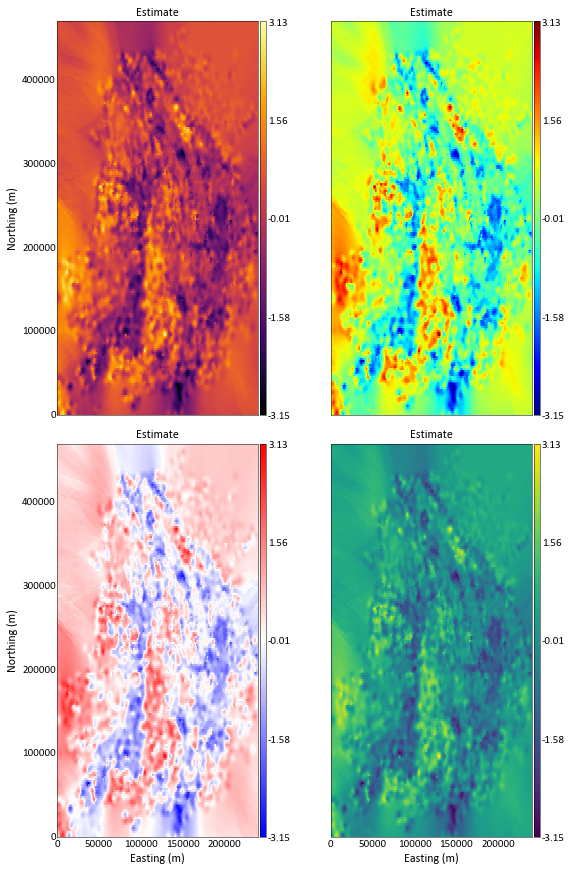
cmaps = ['inferno', 'jet', 'bwr', 'viridis']
fig, axes = gs.subplots(2, 2, axes_pad=(0.9, 0.4), figsize= (20,15), cbar_mode='each', label_mode='L')
for i, ax in enumerate(axes):
    gs.slice_plot(krigfl, var='Estimate', orient='xy', cmap=cmaps[i], ax=ax)
[ ]:
# Clean up
try:
    gs.rmfile('kt3dn.sum')
    gs.rmfile('kt3dn.dbg')
    gs.rmfile('kt3dn_dataspacing.out')
    gs.rmfile('temp')
    gs.rmdir(outdir)
except:
    pass