

Python and pygeostat#
Introduction#
This notebook gives a brief overview of python and pygeostat for researchers and affiliates of CCG. This notebook is not an introduction to python in general, but is designed to help with:
deciding whether using python would be valuable for your work
applying python to geostatistics problems using CCG and GSLIB software
the basics of using python and pygslib to analyze data, visualize results and interface with Paraview
Python is an interpreted, high level general purpose programming and scripting language which is very well suited to many of the common scripting tasks where bash or matlab would typically be used, and many tasks where an entire Fortran program might have previously been used. The huge collection of libraries for python covering machine learning, statistics, data management and optimization make it very useful for geostatistical workflows. There are many excellent tutorials for Python available which do a much better job introducing the language than this notebook would.
Pygeostat is a python module using fortran libraries which was written to facilitate working with GeoEAS data files (GSLIB format), CSV data files, and GSLIB and CCG software. The integrated fortran libraries making pygeostat extremely quick to use for many applications, such as variogram calculation and modeling requiring no parameter files. For other GSLIB and CCG programs, generic interface routines are provided to interface with the programs using standard string interpolation techniques familiar to anyone who has scripted with Bash.
Running this notebook#
If you wish to run the code in this notebook yourself, a scientific python distribution and pygeostat are required. Otherwise, all output is shown in the notebook below each cell so you can see the output without install python and running the notebook yourself. The Anaconda distribution of Python is recommended and is compatible with Windows, Mac and unix distributions.
To quickly setup python and pygeostat:
Download and run the Anaconda graphical installer of Python 3.* from http://continuum.io/downloads. Have the installer add python to the path. Test that the install worked by opening up a command prompt (cygwin or cmd) and running ‘python –version’. The install version should be reported.
Install pygeostat using Python packaging Index (PyPI)
pip install pygeostat
Follow the examples provided in this document
Center for Computational Geostatistics (CCG)
[ ]:
import os, sys
import pygeostat as gs
import matplotlib.pyplot as plt

exe_dir="../pygeostat/executable/"
Brief Introduction to Python#
An extremely quick introduction to python is given here. Python is a high level interpreted programming language. Variable assignment and math is simple. The print operator prints to the screen. Whitespace (in the form of 4 spaces) is used for blocks such as if statements, or loops.
[ ]:
print('Hello World!')

print('Math is easy and works as expected')
a = 1
b = 2
print('a =',a,'b =',b)
print('a + b =',a+b)
print('a/b+0.2 =',a/b+0.2)

if (1>2):
    print('This statement is unreachable')
else:
    print('Note the 4 spaces for block statements like if and loops')

print('Loops can use a list, or a range among other things!')
for i in [1,2,10]:
    print(i)

print('Note that everything starts from 0 in python unlike Fortran')
for i in range(3):
    print(i)


mystr = 'Hello World!'
print('Lots of helpful options are built in such as string splitting:',mystr.split())
Hello World!
Math is easy and works as expected
a = 1 b = 2
a + b = 3
a/b+0.2 = 0.7
Note the 4 spaces for block statements like if and loops
Loops can use a list, or a range among other things!
1
2
10
Note that everything starts from 0 in python unlike Fortran
0
1
2
Lots of helpful options are built in such as string splitting: ['Hello', 'World!']
[ ]:
c, d = 2.561, 10.2
print('c = {}, d = {}'.format(c, d))
print('c = {:.1f}, d = {:.2e}'.format(c, d))
c = 2.561, d = 10.2
c = 2.6, d = 1.02e+01
Pygeostat Parameters and Matplotlib PlotStyle#
Pygeostat allows for default settings to be specified. This provides added convenience, since many arguments may be left to defaults and not specified repeatedly throughout the course of a notebook/project.
Also, pygeostat has a default PlotStyle that uses Matplotlib’s rcParams dictionary to setup a consistent plot style throughout the course of a notebook/project.
[ ]:
# Setting the cat dictionary
gs.Parameters['data.catdict'] = {1: 'Inside', 0: 'Outside'}
gs.Parameters.describe('data.catdict')
data.catdict:
When initializing a DataFile, this dictionary will be used as DataFile.catdict (if catdict.keys() matches DataFile.cat codes). This dictionary is formaatted as {catcodes: catnames}.
[ ]:
gs.Parameters
Parameters({'config.autoload.parameters': True,
            'config.autoload.plot_style': False,
            'config.getpar': False,
            'config.ignore_mpl_warnings': True,
            'config.nprocess': 4,
            'config.verbose': True,
            'data.cat': None,
            'data.catdict': {0: 'Outside', 1: 'Inside'},
            'data.dh': None,
            'data.fix_legacy_null': False,
            'data.griddef': None,
            'data.ifrom': None,
            'data.io.pandas_engine': 'python',
            'data.ito': None,
            'data.legacy_null': [-999, -998, -99, -98],
            'data.nreal': None,
            'data.null': -999.0,
            'data.null_vtk': 0.0,
            'data.tmin': -998.0,
            'data.weights': None,
            'data.write.python_floatfmt': '%.6f',
            'data.write_vtk.cdtype': 'float64',
            'data.write_vtk.vdtype': 'float64',
            'data.x': None,
            'data.y': None,
            'data.z': None,
            'plotting.assumecat': 11,
            'plotting.axis_xy': False,
            'plotting.axis_xy_spatial': False,
            'plotting.cmap': 'viridis',
            'plotting.cmap_cat': 'tab20',
            'plotting.gammasize': 3.0,
            'plotting.grid': False,
            'plotting.histogram_plot.cdfcolor': '.5',
            'plotting.histogram_plot.edgecolor': 'k',
            'plotting.histogram_plot.edgeweight': None,
            'plotting.histogram_plot.facecolor': '.9',
            'plotting.histogram_plot.histbins': 15,
            'plotting.histogram_plot.stat_blk': 'all',
            'plotting.histogram_plot.stat_xy': [0.95, 0.95],
            'plotting.histogram_plot.stat_xy_cdf': [0.95, 0.05],
            'plotting.histogram_plot_simulation.alpha': 0.5,
            'plotting.histogram_plot_simulation.refclr': 'C3',
            'plotting.histogram_plot_simulation.simclr': '0.2',
            'plotting.lagname': 'Lag Distance',
            'plotting.location_plot.c': '.4',
            'plotting.location_plot.lw': 5.0,
            'plotting.location_plot.s': 20.0,
            'plotting.log_lowerval': 0.0001,
            'plotting.nticks': None,
            'plotting.rotateticks': [0, 0],
            'plotting.roundstats': True,
            'plotting.scatter_plot.alpha': 1.0,
            'plotting.scatter_plot.c': 'kde',
            'plotting.scatter_plot.cmap': 'viridis',
            'plotting.scatter_plot.s': None,
            'plotting.scatter_plot.stat_blk': 'pearson',
            'plotting.scatter_plot.stat_xy': [0.95, 0.05],
            'plotting.sigfigs': 2,
            'plotting.stat_fontsize': None,
            'plotting.stat_ha': 'right',
            'plotting.stat_linespacing': 1.0,
            'plotting.unit': 'm',
            'plotting.variogram_plot.color': '.5',
            'plotting.variogram_plot.ms': 6.0,
            'plotting.variogram_plotsim.alpha': 0.5,
            'plotting.variogram_plotsim.refclr': 'C3',
            'plotting.variogram_plotsim.simclr': '0.2',
            'plotting.vplot.colors': ['C0', 'C1', 'C2'],
            'plotting.xabbrev': 'E',
            'plotting.xname': 'Easting',
            'plotting.yabbrev': 'N',
            'plotting.yname': 'Northing',
            'plotting.zabbrev': 'Elev',
            'plotting.zname': 'Elevation'})
[ ]:
gs.Parameters['data.griddef'] = gs.GridDef('''
120 5.0 10.0
110 1205.0 10.0
1 0.5 1.0''')
print(gs.Parameters['data.griddef'])
gs.Parameters.describe('data.griddef')
120 5.0 10.0
110 1205.0 10.0
1 0.5 1.0
data.griddef:
When initializing a DataFile, this will be used as DataFile.GridDef if GridDef.count() matches DataFile.shape[0]. A pygeostat.GridDef object or valid gridstr/gridarr may be used for intitialization.
[ ]:
# Default plot settings
gs.PlotStyle['font.size'] = 12
gs.PlotStyle['figure.figsize'] = (10, 10)
Importing GSLIB files to python with pygeostat#
We will use the oilsands training data set for this example. A pygeostat DataFile object is used to store the data, and relevant parameters such as the names of x, y and z coordinates. The DataFile class stores data by default in a Pandas DataFrame called ‘data’.
Pygeostat contains a collection of example data sets under ~:nbsphinx-math:pygeostat\data\example_data that can be access through ExampleData.
[ ]:
datafl = gs.ExampleData('oilsands')
datafl.head()
| Drillhole Number | East | North | Elevation | Bitumen | Fines | Chlorides | Facies Code | |
|---|---|---|---|---|---|---|---|---|
| 0 | 2.0 | 1245.0 | 10687.09 | 257.5 | 7.378 | 28.784 | -9.0 | -9.0 |
| 1 | 2.0 | 1245.0 | 10687.09 | 254.5 | 9.176 | 22.897 | -9.0 | -9.0 |
| 2 | 2.0 | 1245.0 | 10687.09 | 251.5 | 11.543 | 15.144 | -9.0 | -9.0 |
| 3 | 2.0 | 1245.0 | 10687.09 | 248.5 | 6.808 | 30.598 | -9.0 | -9.0 |
| 4 | 2.0 | 1245.0 | 10687.09 | 245.5 | 10.657 | 18.011 | -9.0 | -9.0 |
[ ]:
datafl.describe()
| Bitumen | Fines | Chlorides | |
|---|---|---|---|
| count | 5808.000000 | 5808.000000 | 5808.000000 |
| mean | 7.708852 | 28.707298 | 103.139353 |
| std | 5.136709 | 21.247085 | 286.545409 |
| min | 0.000000 | 0.861000 | -9.000000 |
| 25% | 2.877750 | 10.166000 | -9.000000 |
| 50% | 7.480000 | 24.453000 | 5.400000 |
| 75% | 12.666000 | 42.823250 | 63.900000 |
| max | 18.428000 | 86.777000 | 2602.000000 |
[ ]:
datafl.variables
['Bitumen', 'Fines', 'Chlorides']
[ ]:
datafl.xyz
['East', 'North', 'Elevation']
Saving data to CSV, HDF5, and VTK file formats#
Working with data is only useful if it can be saved.
[ ]:
out_dir = 'Output'
gs.mkdir(out_dir)

outgslibfl = os.path.join(out_dir,'oilsands_out.dat')
outcsvfl = os.path.join(out_dir,'oilsands_out.csv')
outhdf5fl = os.path.join(out_dir,'oilsands_out.hdf5')

print('\nThe datafile can be saved as a GSLIB file:',outgslibfl)
datafl.write_file(flname=outgslibfl, fltype='GSLIB')

print('\nOr as a hdf5 file which can be opened by Excel')
print('A subset of columns, can be saved with any of these modes - just saving X, Y and Z for example:',outhdf5fl)
datafl.write_file(flname=outhdf5fl, variables=['East','North','Elevation'])

print('\nOr as a CSV file which can be opened by Excel')
print('A subset of columns, can be saved with any of these modes - just saving X, Y and Z for example:',outcsvfl)
datafl.write_file(flname=outcsvfl, variables=['East','North','Elevation'], fltype='CSV')
The datafile can be saved as a GSLIB file: Output\oilsands_out.dat

Or as a hdf5 file which can be opened by Excel
A subset of columns, can be saved with any of these modes - just saving X, Y and Z for example: Output\oilsands_out.hdf5

Or as a CSV file which can be opened by Excel
A subset of columns, can be saved with any of these modes - just saving X, Y and Z for example: Output\oilsands_out.csv
[ ]:
outvtkfl = os.path.join(out_dir,'oilsands_out.vtk')

print('\nThe datafile can be saved as a VTK file:',outvtkfl)
datafl.write_file(flname=outvtkfl, fltype='VTK')
The datafile can be saved as a VTK file: Output\oilsands_out.vtk
Data Visualization using Pygeostat#
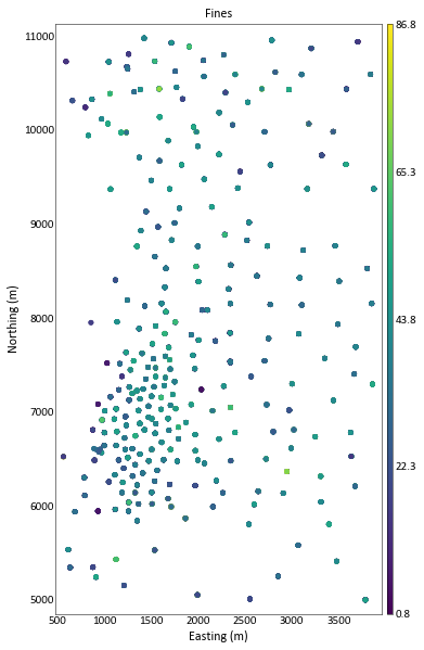
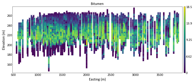
Explore the spatial aspect of the data using location_plot
[ ]:
datafl = gs.DataFile(outgslibfl)
gs.location_plot(datafl, var='Fines')
<mpl_toolkits.axes_grid1.axes_divider.LocatableAxes at 0x16a10706f98>
[ ]:
gs.location_plot(datafl, var='Bitumen', orient='xz', aspect = 10)
<mpl_toolkits.axes_grid1.axes_divider.LocatableAxes at 0x16a106468d0>
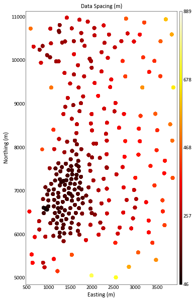
Calculate and visualize data spacing
[ ]:
datafl.spacing(n_nearest=5)
datafl.head()
| Drillhole Number | East | North | Elevation | Bitumen | Fines | Chlorides | Facies Code | Data Spacing (m) | |
|---|---|---|---|---|---|---|---|---|---|
| 0 | 2.0 | 1245.0 | 10687.09 | 257.5 | 7.378 | 28.784 | -9.0 | -9.0 | 184.486903 |
| 1 | 2.0 | 1245.0 | 10687.09 | 254.5 | 9.176 | 22.897 | -9.0 | -9.0 | 184.486903 |
| 2 | 2.0 | 1245.0 | 10687.09 | 251.5 | 11.543 | 15.144 | -9.0 | -9.0 | 184.486903 |
| 3 | 2.0 | 1245.0 | 10687.09 | 248.5 | 6.808 | 30.598 | -9.0 | -9.0 | 184.486903 |
| 4 | 2.0 | 1245.0 | 10687.09 | 245.5 | 10.657 | 18.011 | -9.0 | -9.0 | 184.486903 |
[ ]:
gs.location_plot(datafl, var='Data Spacing (m)', s=50, cmap='hot')
<mpl_toolkits.axes_grid1.axes_divider.LocatableAxes at 0x16a1349b5f8>
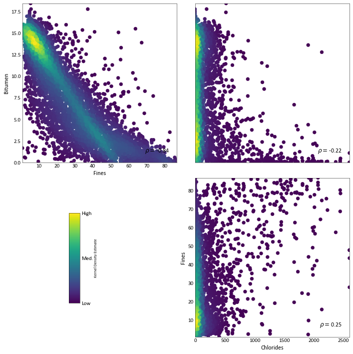
Visulaize multivariate relationships using pygeostat scatter_plots function that infers variables form the data file and calcultae the bivariate KDE
[ ]:
_ = gs.scatter_plots(datafl)
[ ]:
gridstr = '''40  0.5  1    -nx, xmin, xsize
40  0.5  1    -ny, ymin, ysize
40  0.5  1    -nz, zmin, zsize'''
griddef = gs.GridDef(grid_str=gridstr)
krigfl = gs.ExampleData('3d_grid', griddef=griddef)
krigfl.describe()
count    64000.000000
mean         0.021495
std          0.989562
min         -4.050000
25%         -0.666000
50%          0.010000
75%          0.686000
max          3.870000
Name: value, dtype: float64
[ ]:
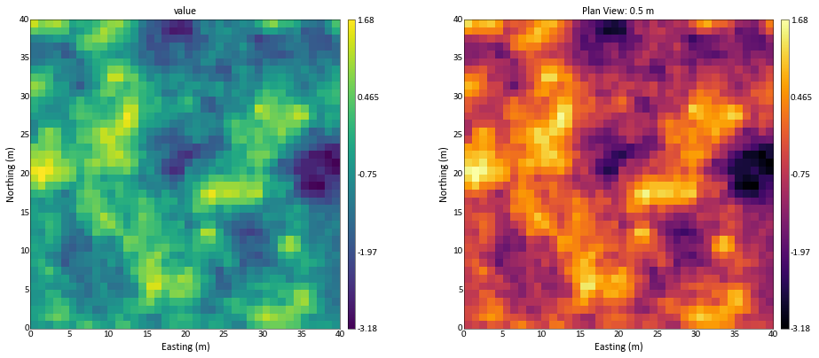
fig, (ax1, ax2) = plt.subplots(1, 2, figsize=(15,15))
plt.subplots_adjust(wspace=0.4)
gs.slice_plot(krigfl, cbar=True, ax=ax1)
gs.slice_plot(krigfl.data['value'], griddef, cbar=True, ax=ax2, cmap='inferno')
<matplotlib.axes._subplots.AxesSubplot at 0x16a14a8eba8>
[ ]:
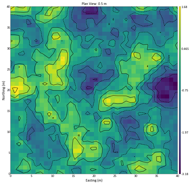
ax = gs.slice_plot(krigfl.data['value'],griddef)
_ = gs.contour_plot(krigfl.data['value'],griddef,ax=ax)
Executing GSLIB programs#
[ ]:
kt3dn = gs.Program(program=exe_dir+'kt3dn', getpar=True)
C:\Users\yimin\Desktop\temp\pygeostat\pygeostat_public\examples\tmpvamdlr98\kt3dn.par has been copied to the clipboard
[ ]:
# use pygeosta to infer grid definition
datafl.infergriddef(blksize=[100,100,10])
Pygeostat GridDef:
34 612.0 100.0
60 5055.0 100.0
14 146.0 10.0
[ ]:
parstr = """                 Parameters for KT3DN
                 ********************
START OF PARAMETERS:
{flname}                         -file with data
{cols}  0                        -  columns for DH,X,Y,Z,var,sec var
-998.0    1.0e21                 -  trimming limits
0                                -option: 0=grid, 1=cross, 2=jackknife
xvk.dat                          -file with jackknife data
1   2   0    3    0              -   columns for X,Y,Z,vr and sec var
kt3dn_dataspacing.out            -data spacing analysis output file (see note)
0    15.0                        -  number to search (0 for no dataspacing analysis, rec. 10 or 20) and composite length
0    100   0                     -debugging level: 0,3,5,10; max data for GSKV;output total weight of each data?(0=no,1=yes)
kt3dn.dbg-nkt3dn.sum             -file for debugging output (see note)
{outfl}                          -file for kriged output (see GSB note)
{griddef}
1    1      1                    -x,y and z block discretization
4    40    12    1               -min, max data for kriging,upper max for ASO,ASO incr
0      0                         -max per octant, max per drillhole (0-> not used)
8000.0  8000.0  400.0              -maximum search radii
 0.0   0.0   0.0                 -angles for search ellipsoid
1                                -0=SK,1=OK,2=LVM(resid),3=LVM((1-w)*m(u))),4=colo,5=exdrift,6=ICCK
0.0  0.6  0.8                  -  mean (if 0,4,5,6), corr. (if 4 or 6), var. reduction factor (if 4)
0 0 0 0 0 0 0 0 0                -drift: x,y,z,xx,yy,zz,xy,xz,zy
0                                -0, variable; 1, estimate trend
extdrift.out                     -gridded file with drift/mean
4                                -  column number in gridded file
onfile                       -gridded file with keyout (see note)
0    1                           -  column (0 if no keyout) and value to keep
2    0.0                      -nst, nugget effect
1    0.25  0.0   0.0   0.0    -it,cc,ang1,ang2,ang3
        400.0  300.0  25.0    -a_hmax, a_hmin, a_vert
1    0.75  0.0   0.0   0.0    -it,cc,ang1,ang2,ang3
      800.0 450.0  30.0    -a_hmax, a_hmin, a_vert
"""

griddef = datafl.griddef

kriging_output = os.path.join(out_dir, 'kt3dn.out')

kt3dnpars ={'flname':datafl.flname,
            'griddef':griddef,
            'outfl': kriging_output,
            'cols':datafl.gscol([datafl.dh]+datafl.xyz + ['Bitumen'])}
print('Note that the string representation of columns can be returned using the GSCOL function for a list of variables:',
      kt3dnpars['cols'])

kt3dn.run(parstr=parstr.format(**kt3dnpars))
Note that the string representation of columns can be returned using the GSCOL function for a list of variables: 1 2 3 4 5
Calling:  ['../pygeostat/executable/kt3dn', 'temp']

 KT3DN Version: 7.4.1

  data file = Output\oilsands_out.dat
  columns =            1           2           3           4           5
           0
  trimming limits =   -998.000000000000       1.000000000000000E+021
  kriging option =            0
  jackknife data file = xvk.dat
  columns =            1           2           0           3           0
  data spacing analysis output file = kt3dn_dataspacing.out
  debugging level =            0
  summary only file = kt3dn.sum
  debugging file = kt3dn.dbg
  GSLIB-style output file = Output\kt3dn.out
  nx, xmn, xsiz =           34   612.000000000000        100.000000000000
  ny, ymn, ysiz =           60   5055.00000000000        100.000000000000
  nz, zmn, zsiz =           14   146.000000000000        10.0000000000000
  block discretization:           1           1           1
  ndmin,ndmax =            4          40
  max per octant =            0
  max per drillhole =            0
  search radii =    8000.00000000000        8000.00000000000
   400.000000000000
  search anisotropy angles =   0.000000000000000E+000  0.000000000000000E+000
  0.000000000000000E+000
   not running data spacing analysis
  using ordinary kriging
  drift terms =            0           0           0           0           0
           0           0           0           0
  itrend =            0
  external drift file = extdrift.out
  GSLIB-style external grid file = extdrift.out
  column for external variable =            4
  keyout indicator file = onfile
  not applying keyout
  nst, c0 =            2  0.000000000000000E+000
  it,cc,ang[1,2,3];            1  0.250000000000000       0.000000000000000E+000
  0.000000000000000E+000  0.000000000000000E+000
  a1 a2 a3:    400.000000000000        300.000000000000
   25.0000000000000
  it,cc,ang[1,2,3];            1  0.750000000000000       0.000000000000000E+000
  0.000000000000000E+000  0.000000000000000E+000
  a1 a2 a3:    800.000000000000        450.000000000000
   30.0000000000000
 Checking the data set for duplicates
  No duplicates found
 Data for KT3D: Variable number            5
   Number   =         5808
   Average  =    7.70885227272725
   Variance =    26.3812369792103
 Presorting the data along an arbitrary vector
 Data was presorted with angles:   12.5000000000000        12.5000000000000
   12.5000000000000
 Setting up rotation matrices for variogram and search
 Setting up super block search strategy

 Working on the kriging
   currently on estimate      2856
   currently on estimate      5712
   currently on estimate      8568
   currently on estimate     11424
   currently on estimate     14280
   currently on estimate     17136
   currently on estimate     19992
   currently on estimate     22848
   currently on estimate     25704
   currently on estimate     28560

 KT3DN Version:    7.4.1 Finished
[ ]:
krigfl = gs.DataFile(kriging_output, griddef=datafl.griddef)
krigfl.head()
| Estimate | EstimationVariance | |
|---|---|---|
| 0 | 2.984331 | 1.138133 |
| 1 | 3.692389 | 1.142133 |
| 2 | 3.785876 | 1.158344 |
| 3 | 3.422368 | 1.166209 |
| 4 | 3.216756 | 1.158588 |
[ ]:
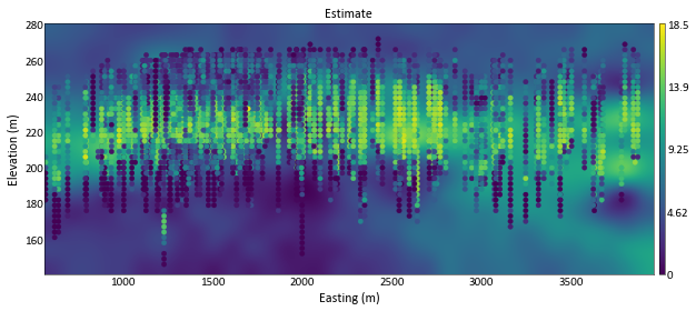
gs.slice_plot(krigfl, var='Estimate', orient='xz', pointdata=datafl, pointvar='Bitumen', aspect = 10)
<mpl_toolkits.axes_grid1.axes_divider.LocatableAxes at 0x16a105be5f8>
[ ]:
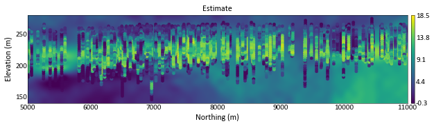
gs.slice_plot(krigfl, var='Estimate', orient='yz', pointdata=datafl, pointvar='Bitumen', aspect = 10)
<mpl_toolkits.axes_grid1.axes_divider.LocatableAxes at 0x16a14d2f1d0>
[ ]:
# Clean up
try:
    gs.rmfile('temp')
    gs.rmfile('kt3dn.dbg')
    gs.rmdir(out_dir) #command to delete generated data file
except:
    pass
[ ]: