Plotting Gallery

PyGeoStat provides a comprehensive library of plotting functions for geostatistical data analysis and visualization. This gallery showcases the main plotting capabilities.

See also

For detailed documentation of each function, see the Plotting API Reference.

---

Statistical Plots

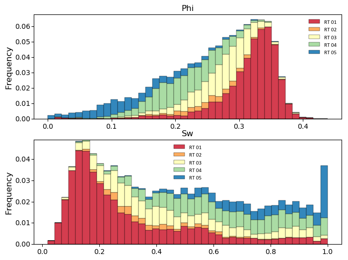
histogram_plot

Standard histogram with optional CDF overlay and summary statistics.

../api/plotting.html#pygeostat.plotting.histogram_plot

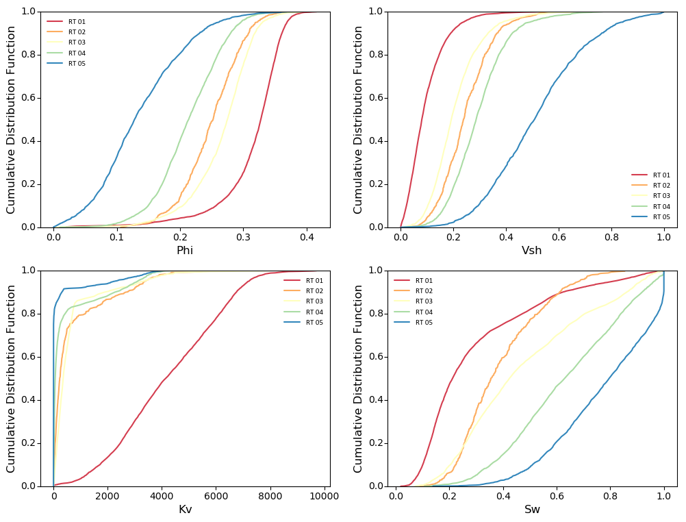
histogram_plot (weighted)

Histogram with weighted data and custom styling.

../api/plotting.html#pygeostat.plotting.histogram_plot

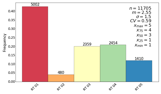
histogram_plot (log scale)

Logarithmic histogram for skewed distributions.

../api/plotting.html#pygeostat.plotting.histogram_plot

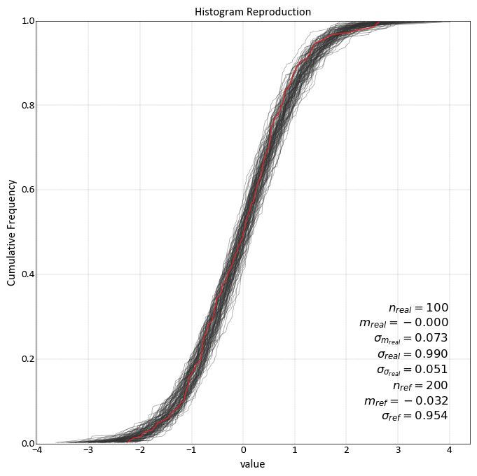
histogram_plot_simulation

Compare multiple realizations against reference data.

../api/plotting.html#pygeostat.plotting.histogram_plot_simulation

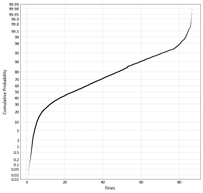
probability_plot

Probability plot for distribution analysis.

../api/plotting.html#pygeostat.plotting.probability_plot

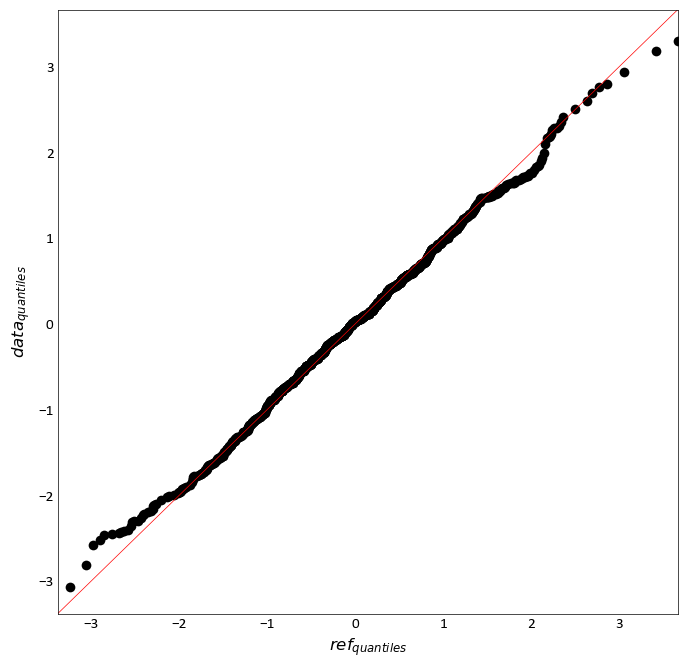
qq_plot

Quantile-quantile plot for comparing distributions.

../api/plotting.html#pygeostat.plotting.qq_plot

---

Scatter & Correlation Plots

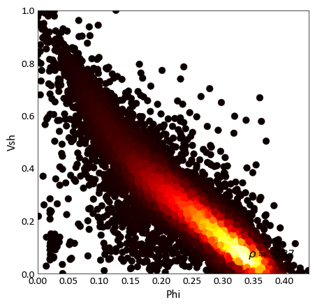
scatter_plot

Basic scatter plot with correlation statistics.

../api/plotting.html#pygeostat.plotting.scatter_plot

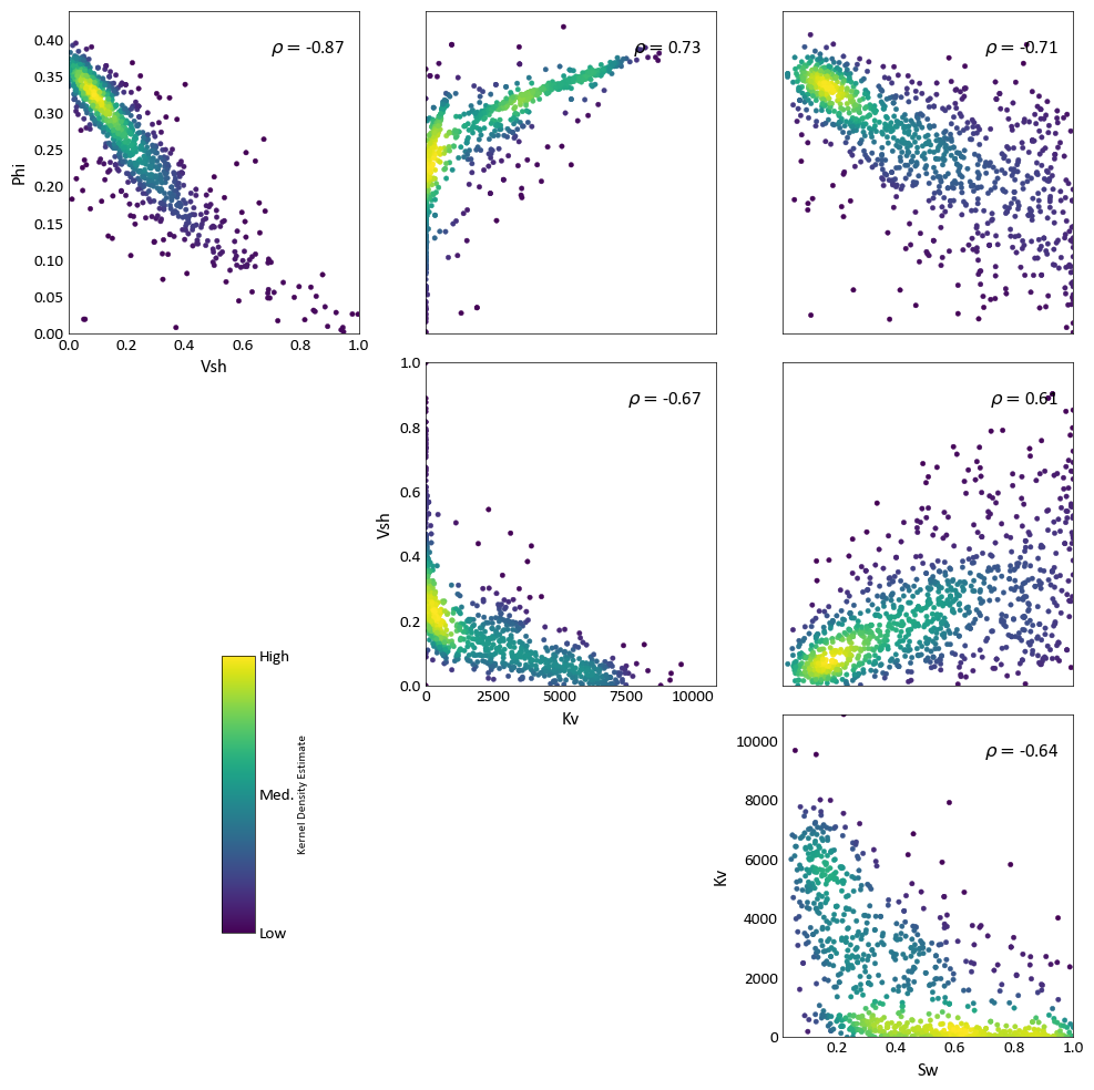
scatter_plots

Matrix of scatter plots for multiple variables.

../api/plotting.html#pygeostat.plotting.scatter_plots

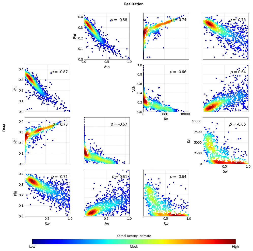
scatter_plots_lu

Lower-upper triangle scatter plot matrix.

../api/plotting.html#pygeostat.plotting.scatter_plots_lu

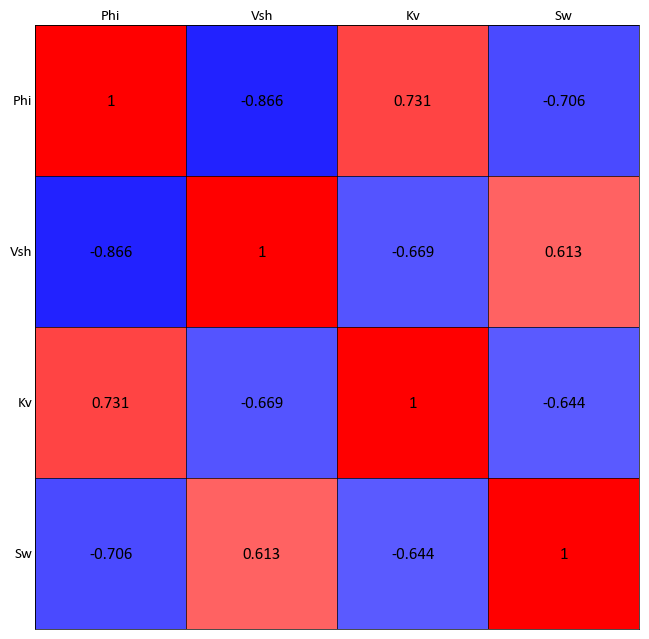
correlation_matrix_plot

Correlation matrix heatmap visualization.

../api/plotting.html#pygeostat.plotting.correlation_matrix_plot

---

Spatial Plots

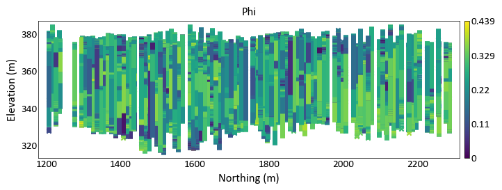
location_plot

Plot spatial data at sample locations.

../api/plotting.html#pygeostat.plotting.location_plot

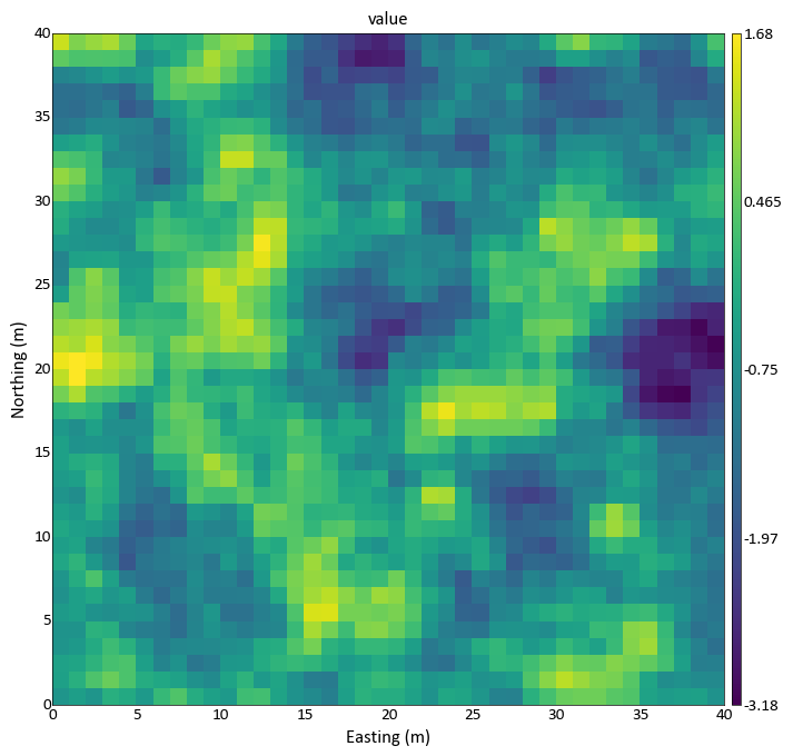
slice_plot

2D slice through 3D spatial data.

../api/plotting.html#pygeostat.plotting.slice_plot

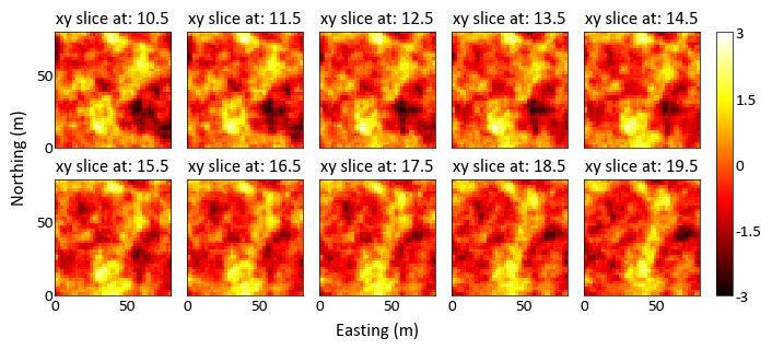
grid_slice_plot

Gridded data slice visualization.

../api/plotting.html#pygeostat.plotting.grid_slice_plot

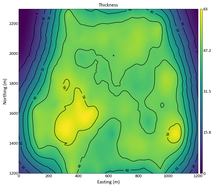
contour_plot

Contour plot for spatial data.

../api/plotting.html#pygeostat.plotting.contour_plot

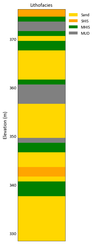
drill_plot

Drillhole log visualization.

../api/plotting.html#pygeostat.plotting.drill_plot

---

Geostatistical Plots

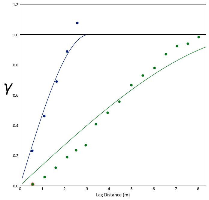
variogram_plot

Experimental and model variogram display.

../api/plotting.html#pygeostat.plotting.variogram_plot

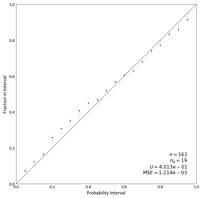
accuracy_plot

Accuracy assessment for estimates.

../api/plotting.html#pygeostat.plotting.accuracy_plot

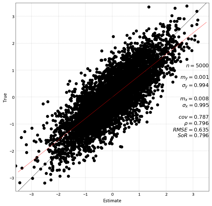
validation_plot

Cross-validation results visualization.

../api/plotting.html#pygeostat.plotting.validation_plot

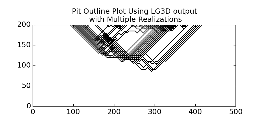
pit_plot

Probability integral transform (PIT) plot.

../api/plotting.html#pygeostat.plotting.pit_plot

---

Multivariate Analysis

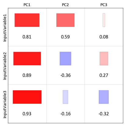
loadings_plot

Factor loadings visualization for PCA/FA.

../api/plotting.html#pygeostat.plotting.loadings_plot

---

Getting Started with Plotting

Basic Example

import pygeostat as gs

# Load example data
data = gs.ExampleData('oilsands')

# Create a histogram
gs.histogram_plot(data, var='Bitumen')

# Create a location plot
gs.location_plot(data, var='Bitumen',
                 x='Easting', y='Northing')

# Create a scatter plot
gs.scatter_plot(data, var1='Bitumen', var2='Fines')

Customizing Plots

Configure default plotting styles using Parameters:

import pygeostat as gs

# Set global plotting parameters
gs.Parameters['plotting.cmap'] = 'viridis'
gs.Parameters['plotting.unit'] = 'm'
gs.Parameters['plotting.xname'] = 'Easting'
gs.Parameters['plotting.yname'] = 'Northing'

# All plots will now use these defaults
gs.location_plot(data, var='Grade')

Saving Figures

import pygeostat as gs

# Create plot and get figure handle
fig, ax = gs.histogram_plot(data, var='Grade')

# Save to file
fig.savefig('histogram.png', dpi=300, bbox_inches='tight')

---

Next Steps

📚 Plotting API Reference

Complete documentation of all plotting functions with parameters and examples.

Plotting Functions

🚀 Getting Started

Introduction to PyGeoStat workflows and basic usage.

Getting Started

🧪 Examples

Complete tutorials demonstrating PyGeoStat in real-world workflows.

Examples

🧩 API Reference

Detailed documentation of all PyGeoStat classes and functions.

API Reference